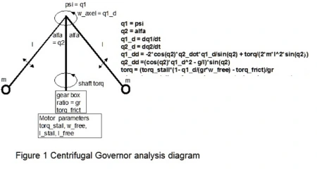
This post derives the equations of motion for a motor driving a variable centrifugal load similar to what one would see on the classical steam engine centrifugal speed governor first invented by James Watt. (Fig 1) Source(https://upload.wikimedia.org/wikipedia/commons/c/c7/Boulton_and_Watt_centrifugal_governor-MJ.jpg)

Non-Feedback Dynamics
We are only concerned here with the response of the engine/centrifugal load without any feedback to the engine from the governor. The analytical diagram for the governor without feedback is:
Typically a motor with a large inertial load has a first order exponential response with a time constant
tau = w_free*I_load/torq_max*gr^2
where w_free is the motor free speed , torq_max is the stall torque of the motor and gr = gear ratio of output shaft speed / motor speed.
The centrifugal weights change the moment of inertia I_load with output shaft speed hence giving the motor a variable time constant. One can bound the motor response between two exponential responses… one with a tau_min and the other with tau_max where min and max tau are respectively associated with the min and max inertial load which are generally set by the mechanical limits of the governor. The motor current response is nonlinear and more gradual than if operating with the full inertia load. This in turn can keep the motor protection PTC fuses from tripping without explicitly controlling the current through the motor controller.
I will post a simulated response later for a Vex system but first we need the equations of motion.
To find the equations of motion I decided for my review to use the Method of Lagrange. For a given system one needs to compute the Lagrangian, L, from the kinetic energy, T and the potential energy V.
L = T – V
We then obtain a system of differential equations from the following computation for each generalized variable q_i.
d(∂L/∂q_i_d)/dt = ∂L/∂q_i + Q_i
where q_i_d = d(q_i)/dt and Q_i are the generalized non conservative forces doing work on the system along the q_i direction. This is a cook book formula that is often times simpler to use than Newtons force equation F = ma. The resulting equations will be the same with either method. Many good references on Lagrange method can be found with a simple Google search.[reference Wikipedia Euler Lagrange Method]
The generalized variables of interest are :
q1 = psi , the angle that the motor is turning through.
q1_d = w_axel = dpsi/dt , the speed at which the motor is turning the governor axles.
q2 = alpha, the angle of the arm from vertical.
q2_d = w_arm = dalpha/dt , the speed that the arms are moving up and down relative to the vertical.
The mass of the weight on one arm is m and the length of the arm is l. Moments of inertia relative the pivots are I_axel and I_arm. I_arm is constant and I_axle varies due to the movement of the arms.
T = 1/2 * I_axel * (w_axel)^2 + 1/2 * I_arm * (w_arm)^2
V = m*g*l*(1-cos(alpha))
I_axel = m*(l*sin(alpha))^2
I_arm = m*l^2
Substituting for the generalized variables
L = T-V = 1/2*m*(l*sin(q2))^2 *q1_d^2 + 1/2*I_arm*(q2_d)^2 – m*g*l*(1-cos(q2))
∂L/∂q1 = 0;
∂L/∂q1_d = m*l^2*sin(q2)^2*q1_d
∂L/∂q2 = m*l^2*sin(q2)*cos(q2)*q1_d^2 – m*g*l*sin(q2)
∂L/∂q2_d= I_arm*q2_d
Now compute d( ∂L/∂q_d)/dt and set equal to dL/dq + Q where Q are the generalized forces that are non conservative associated with each q.
For q1:
d(m*l^2*sin(q2)^2*q1_d)/dt = m*l^2*(2*sin(q2)*cos(q2)*q2_d*q1_dot + sin(q2)^2*q1_dd) = torq
1) q1_dd = -2*cos(q2)*q2_dot*q1_d/sin(q2) + torq/(m*l^2*sin(q2)^2)
For q2:
I_arm*q2_dd = m*l^2*sin(q2)*cos(q2)*q1_d^2 – m*g*l*sin(q2)
or
2) q2_dd = ( cos(q2)*q1_d^2 – g/l)*sin(q2)
Steady State requirements
In the steady state, q1_dd = q2_dd = q2_dot = o. This then gives the q2 as a function of q1_d or alfa as a function of the axle speed , w_axle.
From equation 2 cos(alfa) = g/(l*w_axle^2)
Since cos(alfa) < =1 the minimum axle speed w_axle_min >=sqrt(g/l) Notice that this requirement is independent of the centrifugal mass very much like a pendulum period is independent of mass and only a function of the pendulum length , l . w_axle_min is the minimum speed before the arms move.
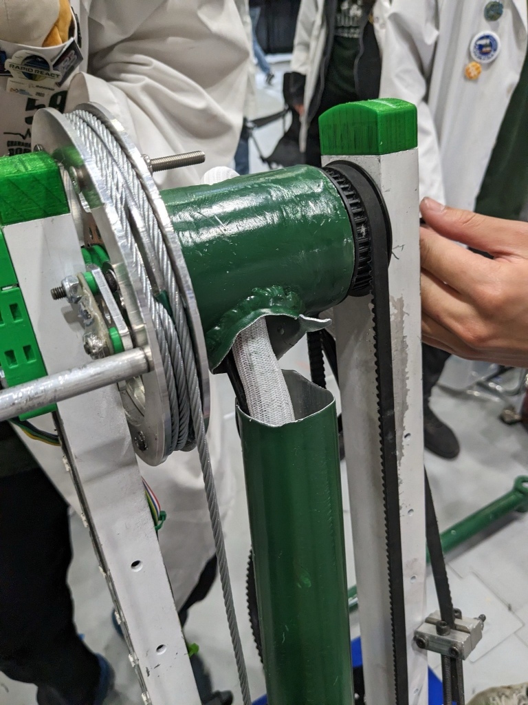
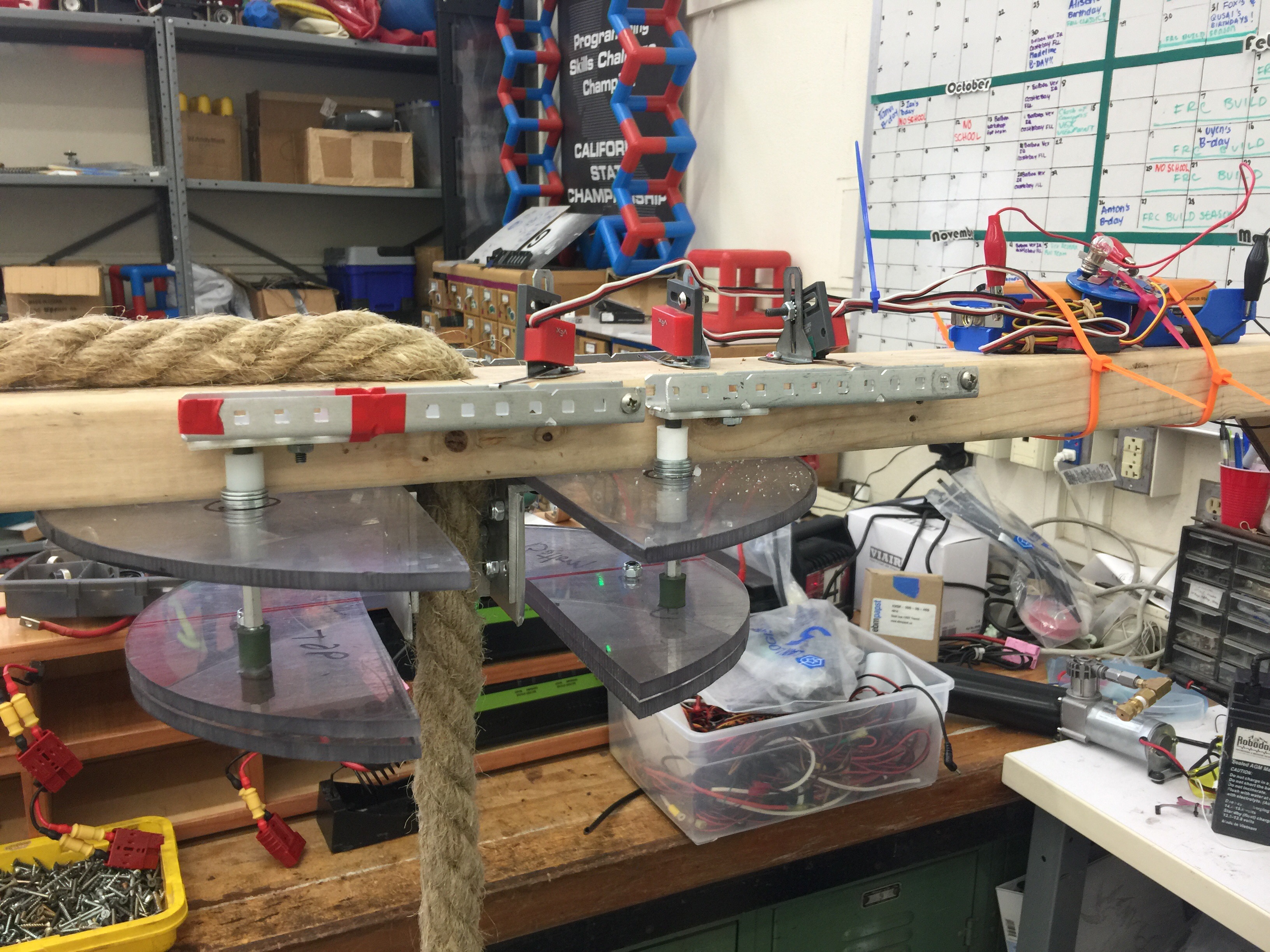
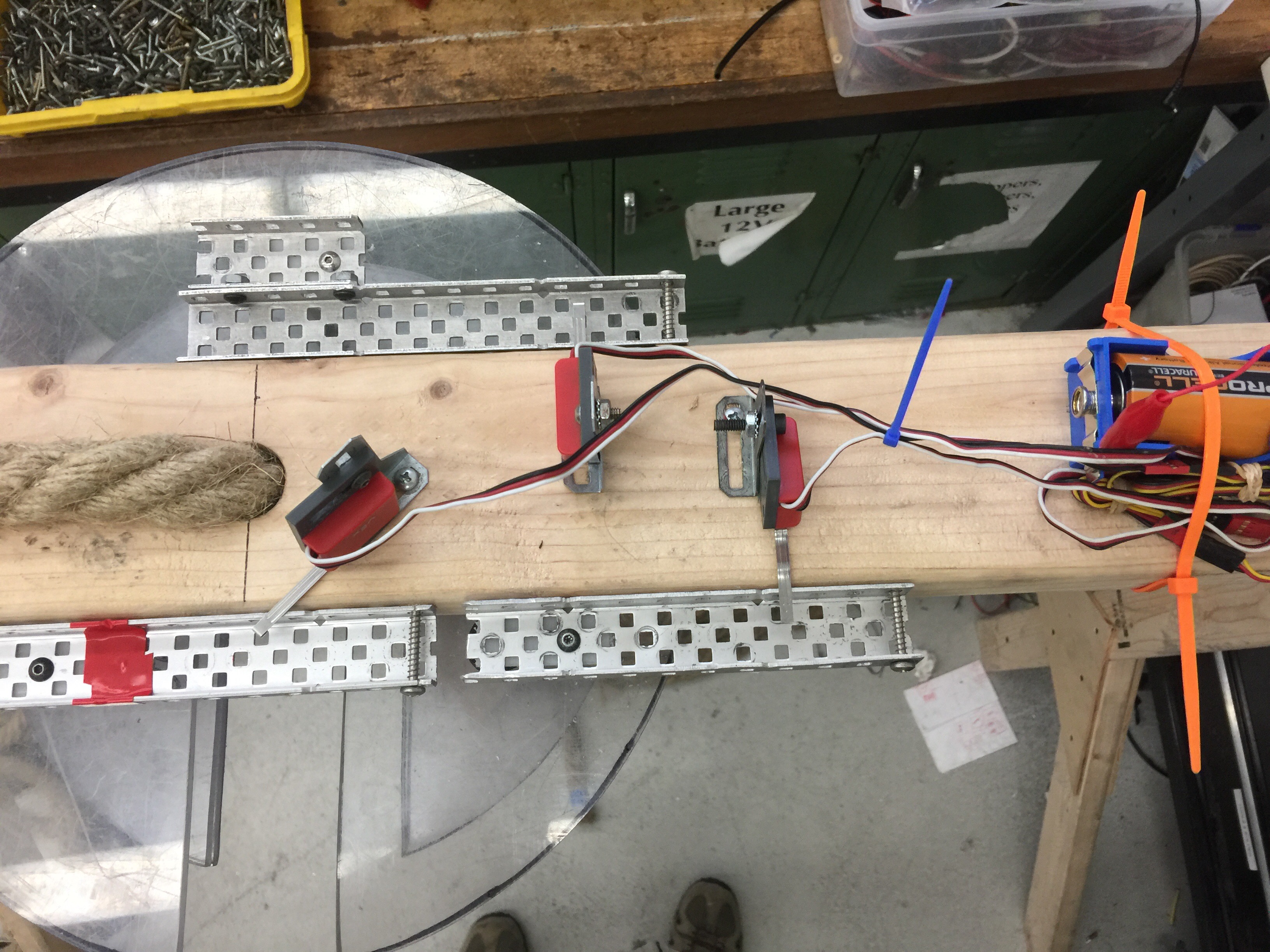
Vex Example
In the Vex centrifugal experimental device shown here , the arms are about 2.5 inches in length so we would expect w_axle_min = sqrt(32.3*12/2.5)= 12.4 rad/s or 118.5 rpm. There appears to be a gearing between the motor and axle of 7 : 1 so the minimum speed of the motor is 118.8/7 =17 rpm which means that the motor driving can be a Vex 393 with standard gearing (100 rpm max). However, there is a mechanical minimum of around 45 degs which means the minimum speed to move is 17 rpm/sqrt(cos(45 deg)) = 20.2 rpm. The speed to fully extend the arms (alpha = 75 deg ?) would be 17 rpm/sqrt(cos(75 deg)) = 33.4 rpm.
System Time constant with alfa = 45 deg and 75 deg.
tau = w_free*I_load*gr^2/torq_max
I am guessing that one arm has a mass of about 1 oz 0r .0283 kg
I_45 = m*(l*sin(alfa))^2 = .o25*(2.5in*.707*.0254 m/in)^2 = 5.038 E-05 kg m^2
I_75 = I_45*(sin(75)/sin(45))^2 = I_45*1.866
tau_45 = w_free*I_45*2*gr^2/torq_max (note: factor of 2 added for two arms)
Since torq_max = 1.67 nm, w_free = 100 rpm*6.28/60 = 10.5 rad/sec , gr = 7
tau_45 = 10.5 * 5.038E-05*2*49/1.67 = .037sec
tau_75 = tau_45*I_75/I/4= .069 sec
Simulated response
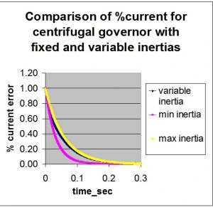
The differential equations were implemented in a simulation to show the time response to a step speed input. The data was generated by my excel program. The red line in the time response shown below is the arm angle starting from 45 deg and quickly moving to 75 deg as the speed increases. This expansion occurs so quickly that most of the motor response is with the maximum moment of inertia. In the second figure, the %current error is shown with fixed and varying moments of inertia.
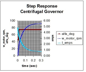
As you can see after about .o2 seconds, the motion of the governor is limited at its maximum alfa = 75 deg and the variable inertia current response (blue curve) is close to the slower fixed inertia response (yellow curve) for most of the current response.
 The o
The o
In this particular experiment, the objective was to keep the current response below the response with the maximum inertia to keep the stress of the motor. In this case the objective was not met. The mass movement was too fast with speed so the governor limited shortly after the initial speed increase. Increasing the length of the arms expands the time scale but doesn’t change the early saturation. One solution would be to add spring tension to the expanding weights so that a higher speed would be required to saturate. This will be addressed later by adding a spring potential energy to the Lagrangian and deriving a new set of equations.


 Posted by vamfun
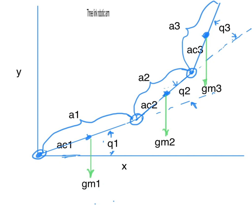


